Fisher RSF
John Fieberg
Preamble
Load libraries
library(ezknitr)
library(knitr)
library(lubridate)
library(raster)
library(move)
library(amt)
library(broom)
library(nlme)
library(lme4)
library(tidyverse)
options(width=165)
opts_chunk$set(fig.width=12,fig.height=4.5, error=TRUE,cache = F)
Read in annotated data.
rsfdat<-read.csv("data/FisherRSF2018-EnvDATA-results.csv")Simplify some variable names
names(rsfdat)[c(4,8:10)]<-c("id","LandClass", "Elevation", "PopDens")
rsfdat$case_<-as.numeric(rsfdat$case_)
Create landcover classes (as suggested by Scott Lapoint :)
rsfdat$LandClass<-as.character(rsfdat$LandClass)
rsfdat<-rsfdat %>% mutate(landC = fct_collapse(LandClass,
      agri = c("11", "14", "30"),
      forest =c("30","40","50","60", "70","80", "90","100"),
      shrub= c("110", "130", "150"),
      grass = c("120", "140"),
      wet= c("160"),
      other = c("170", "180", "190", "200", "210", "220")))
## Warning: Unknown levels in `f`: 11, 14, 40, 60, 80, 90, 150, 170, 180, 200, 220Center and scale variables
rsfdat<-rsfdat %>% mutate(elev=as.numeric(scale(Elevation)),
                          popD=as.numeric(scale(PopDens)))
Explore the data:
Look Distribution of variables for used and available
binomial_smooth <- function(...) {
  geom_smooth(method = "glm", method.args = list(family = "binomial"), ...)
}
ggplot(rsfdat,aes(x=Elevation, y=case_))+
  stat_smooth(method="glm", method.args = list(family = "binomial"))+
  binomial_smooth(formula = y ~ splines::ns(x, 5), colour="red")+
  facet_wrap(~id, scales="free")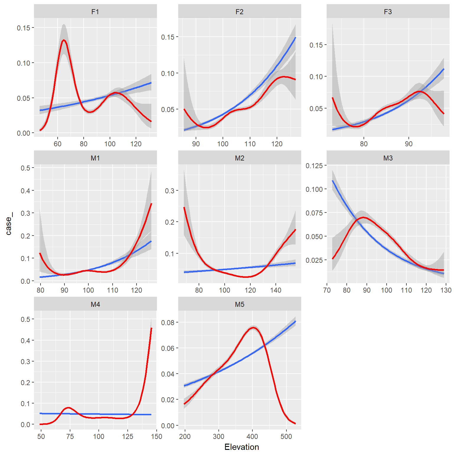
ggplot(rsfdat,aes(x=PopDens, y=case_))+
  stat_smooth(method="glm", method.args = list(family = "binomial"))+
  binomial_smooth(formula = y ~ splines::ns(x, 5), colour="red")+
  facet_wrap(~id, scales="free")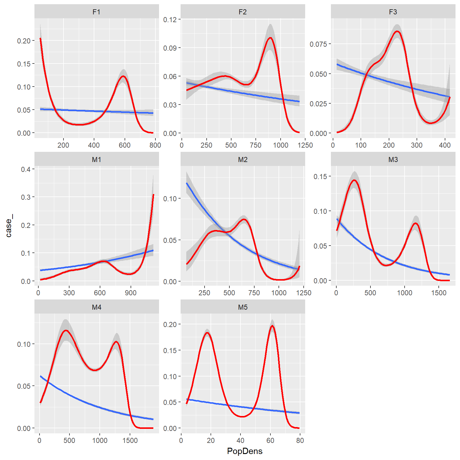
ggplot(rsfdat, aes(x=landC, y=..prop..,group=case_, colour=case_))+
  geom_bar(position="dodge", aes(fill=case_))+facet_wrap(~id, scales="free")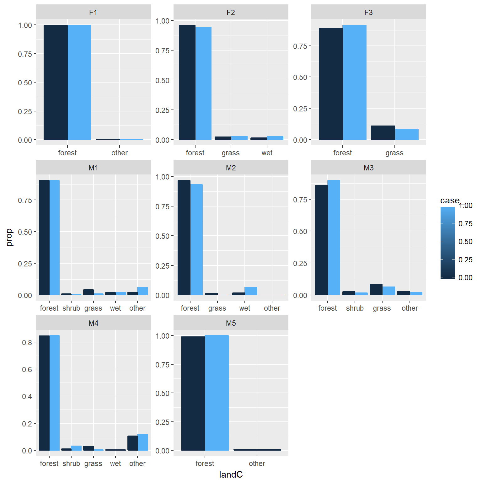
RSF fitting
Weight available data
rsfdat$w<-ifelse(rsfdat$case_==1, 1, 5000)We can fit an RSF model to a single animal using logistic regression
summary(glm(case_ ~ elev+popD+landC, data = subset(rsfdat, id=="M2"), weight=w,family = binomial))##
## Call:
## glm(formula = case_ ~ elev + popD + landC, family = binomial,
## data = subset(rsfdat, id == "M2"), weights = w)
##
## Deviance Residuals:
## Min 1Q Median 3Q Max
## -0.7297 -0.3648 -0.2956 -0.2381 5.3464
##
## Coefficients:
## Estimate Std. Error z value Pr(>|z|)
## (Intercept) -9.27634 0.15652 -59.268 < 2e-16 ***
## elev 2.02810 0.20492 9.897 < 2e-16 ***
## popD -0.73881 0.04234 -17.450 < 2e-16 ***
## landCgrass -3.32900 1.00048 -3.327 0.000877 ***
## landCwet 1.92521 0.10705 17.984 < 2e-16 ***
## landCother -8.25493 90.02876 -0.092 0.926943
## ---
## Signif. codes: 0 '***' 0.001 '**' 0.01 '*' 0.05 '.' 0.1 ' ' 1
##
## (Dispersion parameter for binomial family taken to be 1)
##
## Null deviance: 40797 on 32503 degrees of freedom
## Residual deviance: 40236 on 32498 degrees of freedom
## AIC: 40248
##
## Number of Fisher Scoring iterations: 10Note, this individual did not experience all landcover classes
rsfdat %>% filter(id=="M2") %>% with(table(case_, landC)) ## landC
## case_ forest shrub grass wet other
## 0 29881 0 452 531 2
## 1 1527 0 1 110 0rsfdat$used<-as.factor(rsfdat$case_)
rsfdat$used<-fct_recode(rsfdat$used, "avail"="0", "used"="1")ggplot(subset(rsfdat, id=="M2"), aes(x=landC,group=used))+
geom_bar(position=position_dodge(), aes(y=..prop.., fill = used), stat="count") +
scale_fill_brewer(palette="Paired")+
geom_text(aes( label = scales::percent(..prop..),
y= ..prop.. ), stat= "count", vjust = -.3, position=position_dodge(0.9)) +
labs(y = "Proportion", fill="used", x="Landcover") 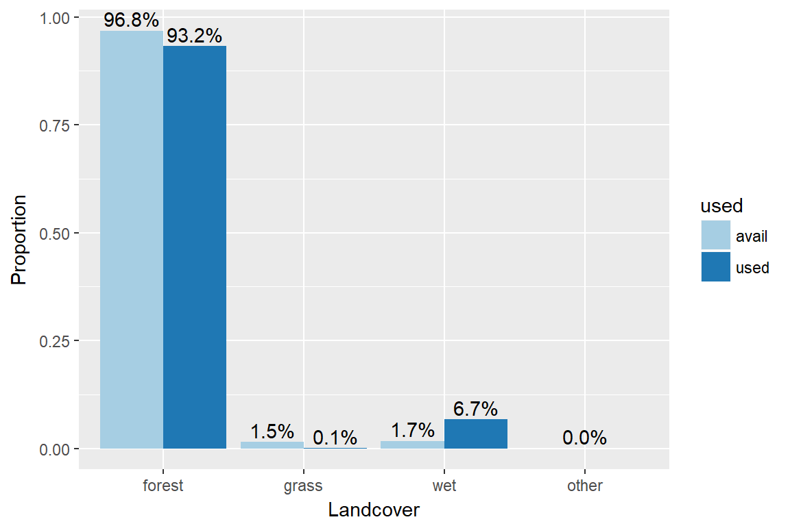
Now, fit an RSF model to data from each animal. Since not all animals experience all habitat types, lets just explore forest versus non-forest
rsfdat$forest<-ifelse(rsfdat$landC=="forest", 1, 0)

fit_rsf <- function(data){
  mod <- glm(case_ ~ elev+popD+forest, data = data, weight=w,family = binomial)
  return(mod)
}
rsffits <- rsfdat %>%  nest(-id) %>%
  dplyr::mutate(mod = purrr::map(data, fit_rsf))
This stores a list of model fits
rsffits ## # A tibble: 8 x 3
## id data mod
## <fct> <list> <list>
## 1 M5 <data.frame [259,207 x 15]> <S3: glm>
## 2 M3 <data.frame [50,198 x 15]> <S3: glm>
## 3 F3 <data.frame [30,956 x 15]> <S3: glm>
## 4 M2 <data.frame [32,504 x 15]> <S3: glm>
## 5 F1 <data.frame [27,797 x 15]> <S3: glm>
## 6 M1 <data.frame [18,935 x 15]> <S3: glm>
## 7 M4 <data.frame [184,587 x 15]> <S3: glm>
## 8 F2 <data.frame [61,183 x 15]> <S3: glm>Look at first model
rsffits$mod[[1]]##
## Call: glm(formula = case_ ~ elev + popD + forest, family = binomial,
## data = data, weights = w)
##
## Coefficients:
## (Intercept) elev popD forest
## -25.3159 0.4674 -2.8697 11.4796
##
## Degrees of Freedom: 259206 Total (i.e. Null); 259203 Residual
## Null Deviance: 326200
## Residual Deviance: 325200 AIC: 325200Now, use tidy to extract information about the model fits into a nested data frame
rsffits <- rsffits %>%
   dplyr::mutate(tidy = purrr::map(mod, broom::tidy),
                 n = purrr::map(data, nrow) %>% simplify())
rsffits
## # A tibble: 8 x 5
## id data mod tidy n
## <fct> <list> <list> <list> <int>
## 1 M5 <data.frame [259,207 x 15]> <S3: glm> <data.frame [4 x 5]> 259207
## 2 M3 <data.frame [50,198 x 15]> <S3: glm> <data.frame [4 x 5]> 50198
## 3 F3 <data.frame [30,956 x 15]> <S3: glm> <data.frame [4 x 5]> 30956
## 4 M2 <data.frame [32,504 x 15]> <S3: glm> <data.frame [4 x 5]> 32504
## 5 F1 <data.frame [27,797 x 15]> <S3: glm> <data.frame [4 x 5]> 27797
## 6 M1 <data.frame [18,935 x 15]> <S3: glm> <data.frame [4 x 5]> 18935
## 7 M4 <data.frame [184,587 x 15]> <S3: glm> <data.frame [4 x 5]> 184587
## 8 F2 <data.frame [61,183 x 15]> <S3: glm> <data.frame [4 x 5]> 61183rsffits$tidy## [[1]]
## term estimate std.error statistic p.value
## 1 (Intercept) -25.3159414 20.37797191 -1.2423190 2.141189e-01
## 2 elev 0.4674258 0.01907326 24.5068620 1.248180e-132
## 3 popD -2.8697109 0.21661498 -13.2479802 4.635108e-40
## 4 forest 11.4795919 20.37770461 0.5633408 5.732029e-01
##
## [[2]]
## term estimate std.error statistic p.value
## 1 (Intercept) -13.7786083 0.28727938 -47.962400 0.000000e+00
## 2 elev -2.6204292 0.34439546 -7.608780 2.766959e-14
## 3 popD -0.4238935 0.02209637 -19.183854 5.049547e-82
## 4 forest 0.5926825 0.06716800 8.823882 1.105585e-18
##
## [[3]]
## term estimate std.error statistic p.value
## 1 (Intercept) -3.3061685 0.83330619 -3.967531 7.262095e-05
## 2 elev 10.2954755 0.98480273 10.454353 1.399505e-25
## 3 popD -0.4269714 0.10935740 -3.904367 9.447249e-05
## 4 forest 0.3742687 0.09371345 3.993756 6.503467e-05
##
## [[4]]
## term estimate std.error statistic p.value
## 1 (Intercept) -8.7696629 0.19534570 -44.893044 0.000000e+00
## 2 elev 1.6098352 0.20464758 7.866378 3.650575e-15
## 3 popD -0.6373201 0.03966744 -16.066581 4.375608e-58
## 4 forest -0.8935558 0.09997356 -8.937921 3.965618e-19
##
## [[5]]
## term estimate std.error statistic p.value
## 1 (Intercept) -11.3605220 1.0394450 -10.929412 8.338737e-28
## 2 elev 1.9774503 0.3115188 6.347772 2.184554e-10
## 3 popD -0.2562964 0.0552215 -4.641243 3.463191e-06
## 4 forest 1.5411823 0.9990089 1.542711 1.229008e-01
##
## [[6]]
## term estimate std.error statistic p.value
## 1 (Intercept) -5.97650776 0.53360729 -11.2001988 4.068196e-29
## 2 elev 7.43464547 0.70103474 10.6052454 2.817233e-26
## 3 popD 0.30794772 0.03873576 7.9499600 1.865717e-15
## 4 forest -0.09290945 0.11327032 -0.8202453 4.120763e-01
##
## [[7]]
## term estimate std.error statistic p.value
## 1 (Intercept) -10.88711842 0.07752620 -140.4314791 0.000000e+00
## 2 elev 0.70694461 0.08487968 8.3287855 8.167591e-17
## 3 popD -0.33340970 0.01252623 -26.6169186 4.324739e-156
## 4 forest -0.01390348 0.03111492 -0.4468427 6.549886e-01
##
## [[8]]
## term estimate std.error statistic p.value
## 1 (Intercept) -5.5085926 0.29189748 -18.871669 1.950419e-79
## 2 elev 7.7095766 0.38596168 19.974980 9.092115e-89
## 3 popD -0.2377759 0.02797363 -8.500001 1.895893e-17
## 4 forest -0.4253830 0.08078356 -5.265712 1.396469e-07Now, create data frame w/ the coefficients, etc
 rsf_coefs <- rsffits %>%
 tidyr::unnest(tidy) %>%
   dplyr::select(-(std.error:p.value))

 rsf_coefs %>% tidyr::spread(term, estimate)
## # A tibble: 8 x 6
## id n `(Intercept)` elev forest popD
## <fct> <int> <dbl> <dbl> <dbl> <dbl>
## 1 F1 27797 -11.4 1.98 1.54 -0.256
## 2 F2 61183 -5.51 7.71 -0.425 -0.238
## 3 F3 30956 -3.31 10.3 0.374 -0.427
## 4 M1 18935 -5.98 7.43 -0.0929 0.308
## 5 M2 32504 -8.77 1.61 -0.894 -0.637
## 6 M3 50198 -13.8 -2.62 0.593 -0.424
## 7 M4 184587 -10.9 0.707 -0.0139 -0.333
## 8 M5 259207 -25.3 0.467 11.5 -2.87Plot coefficients
 rsf_coefs %>% filter(term!="(Intercept)") %>%
   ggplot(., aes(x=1, y=estimate)) +
      geom_dotplot(binaxis="y", stackdir="center")+geom_hline(yintercept=0)+
      facet_wrap(~term, scales="free")
## `stat_bindot()` using `bins = 30`. Pick better value with `binwidth`.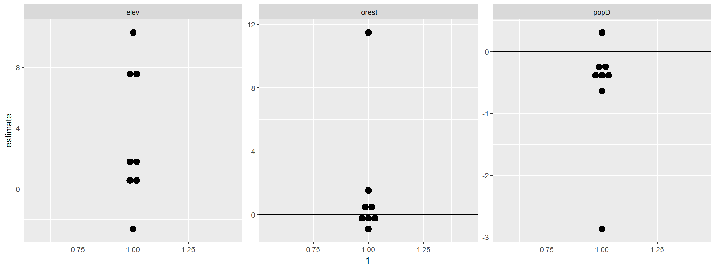
Write out coefficients for MultipleAnimals.R
save(rsf_coefs, file="data/rsfcoefs.Rdata")