TestVignette

Purpose

test whether you have everything set up for the workshop
retrieve and explore animal movement data from Movebank
illustrate how to work with functions in the animal movement tools package (amt)
write out available points for further annotating in EnvDATA

Preamble

Load libraries

library(knitr)
library(lubridate)
library(maptools)
library(raster)
library(move)
library(amt) 
library(ggmap)
library(tibble)
library(leaflet)
library(dplyr)
options(width=165,digits.secs = 3)
opts_chunk$set(fig.width=12,fig.height=4.5, error=TRUE,cache = F)

Record time for running all code

ptm<-proc.time()

Set the seed for the random number generator, so it will be possible to reproduce the random points

set.seed(10299)

Create a login object for a user account at movebank.org

loginStored <- movebankLogin(username="MovebankWorkshop", password="genericuserforthisexercise")

Get overview information about a Movebank study. Be sure to check the citation and license terms if not using your own data.

getMovebankStudy(study="Martes pennanti LaPoint New York", login=loginStored) # see study-level info

##                                                                                                                                                                                                                                                                                                                                                                                                                                                                 acknowledgements
## 1 This work was supported in part by NSF (grant 0756920 to RK), the New York State Museum, \nthe Max Planck Institute for Ornithology; the North Carolina Museum of Natural Sciences, and a National Geographic Society Waitt Grant (SDL).  We thank the Albany Pine Bush Preserve, Dina Dechmann, Neil Gifford, Wolfgang Heidrich, Bart Kranstauber, Franz Kümmeth, Roger Powell, Kamran Safi, Marco Smolla, and Brad Stratton for their logistical support and valuable input.
##   bounding_box
## 1           NA
##                                                                                                                                                                                    citation
## 1 LaPoint, S, Gallery P, Wikelski M, Kays R (2013) Animal behavior, cost-based corridor models, and real corridors. Landscape Ecology, v 28 i 8, p 1615–1630. doi:10.1007/s10980-013-9910-0
##   comments enable_for_animal_tracker                                                                                              grants_used has_quota i_am_owner
## 1       NA                        NA National Science Foundation (#0756920 to RWK) and the National Geographic Society's Waitt Grant (to SDL)      true      false
##        id
## 1 6925808
##                                                                                                                                                                                                                   license_terms
## 1 These data have been published by the Movebank Data Repository with DOI 10.5441/001/1.2tp2j43g. See www.datarepository.movebank.org/handle/10255/move.328. Please contact the PI prior to use of these data for any purposes.
##   location_description main_location_lat main_location_long                             name number_of_deployments number_of_events number_of_individuals
## 1                   NA          42.75205          -73.86246 Martes pennanti LaPoint New York                    NA               NA                    NA
##   number_of_tags principal_investigator_address principal_investigator_email principal_investigator_name
## 1             NA                             NA                           NA                          NA
##                                                                                                                                                                    study_objective
## 1 To investigate the use of corridors by fisher within a suburban landscape and to validate cost-based corridor model predictions with both animal tracking data and camera traps.
##   study_type suspend_license_terms timestamp_end timestamp_start i_can_see_data there_are_data_which_i_cannot_see
## 1   research                 false            NA              NA           true                             false

You may receive a message that you do not have access to data in a study. If you are not a data manager for a study, the owner may require that you read and accept the license terms once before you may download it. Currently license terms cannot be accepted directly from the move package. To view and accept them, go to movebank.org, search for the study and begin a download, and view and accept the license terms. After that you will be able to load from R. Load data from a study in Movebank and create a MoveStack object. For more details and options see https://cran.r-project.org/web/packages/move/index.html.

fisher.move <- getMovebankData(study="Martes pennanti LaPoint New York", login=loginStored)
head(fisher.move)

##    sensor_type_id behavioural_classification eobs_battery_voltage eobs_fix_battery_voltage eobs_horizontal_accuracy_estimate eobs_key_bin_checksum
## 5             653                                              NA                       NA                                NA                    NA
## 6             653                                              NA                       NA                                NA                    NA
## 7             653                                              NA                       NA                                NA                    NA
## 9             653                                              NA                       NA                                NA                    NA
## 15            653                                              NA                       NA                                NA                    NA
## 16            653                                              NA                       NA                                NA                    NA
##    eobs_speed_accuracy_estimate eobs_start_timestamp eobs_status eobs_temperature eobs_type_of_fix eobs_used_time_to_get_fix ground_speed heading
## 5                            NA                   NA          NA               NA               NA                        80           NA      NA
## 6                            NA                   NA          NA               NA               NA                         7           NA      NA
## 7                            NA                   NA          NA               NA               NA                        58           NA      NA
## 9                            NA                   NA          NA               NA               NA                        90           NA      NA
## 15                           NA                   NA          NA               NA               NA                        71           NA      NA
## 16                           NA                   NA          NA               NA               NA                        57           NA      NA
##    height_above_ellipsoid location_lat location_long manually_marked_outlier               timestamp               update_ts deployment_id  event_id  tag_id
## 5                      NA     42.79528     -73.86015                      NA 2011-02-11 18:06:13.999 1970-01-01 00:00:00.000       8623923 170635812 8623917
## 6                      NA     42.79534     -73.86001                      NA 2011-02-11 18:10:08.999 1970-01-01 00:00:00.000       8623923 170635813 8623917
## 7                      NA     42.79528     -73.86013                      NA 2011-02-11 18:20:58.997 1970-01-01 00:00:00.000       8623923 170635814 8623917
## 9                      NA     42.79483     -73.86012                      NA 2011-02-11 18:41:30.999 1970-01-01 00:00:00.000       8623923 170635816 8623917
## 15                     NA     42.79509     -73.86037                      NA 2011-02-11 19:41:10.997 1970-01-01 00:00:00.000       8623923 170635822 8623917
## 16                     NA     42.79515     -73.86023                      NA 2011-02-11 19:50:58.000 1970-01-01 00:00:00.000       8623923 170635823 8623917
##    sensor_type
## 5          GPS
## 6          GPS
## 7          GPS
## 9          GPS
## 15         GPS
## 16         GPS

Note: If there are duplicate animal-timestamp records in Movebank, you will get a warning. You can exclude duplicate records on import using removeDuplicatedTimestamps=T. If you are a data manager for a study in Movebank you can also filter them out directly in the study so they are excluded by default in downloads (see https://www.movebank.org/node/27252). Create a data frame from the MoveStack object

fisher.dat <- as(fisher.move, "data.frame")

Data cleaning

Delete observations where missing lat or long or a timestamp. There are no missing observations in this data set, but it is still good practice to check.

ind<-complete.cases(fisher.dat[,c("location_lat", "location_long", "timestamp")])
fisher.dat<-fisher.dat[ind==TRUE,]

Check for duplicated observations (ones with same lat, long, timestamp, and individual identifier). There are no duplicate observations in this data set, but it is still good practice to check.

ind2<-fisher.dat %>% select(timestamp, location_long, location_lat, local_identifier) %>%
  duplicated
sum(ind2) # no duplicates

## [1] 0

fisher.dat<-fisher.dat[ind2!=TRUE,]

Make timestamp a date/time variable

fisher.dat$timestamp<-as.POSIXct(fisher.dat$timestamp, format="%Y-%m-%d %H:%M:%OS", tz="UTC")

Look at functions in the move package.

plot(fisher.move)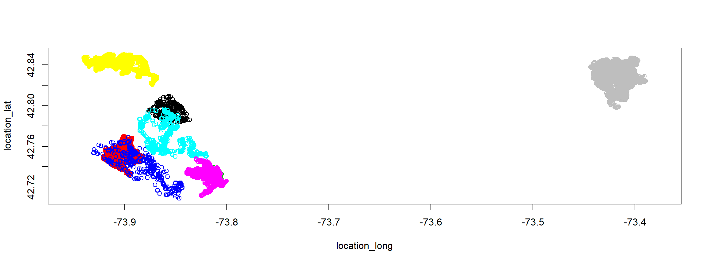

show(fisher.move)

## class       : MoveStack 
## features    : 32904 
## extent      : -73.94032, -73.38947, 42.70898, 42.851  (xmin, xmax, ymin, ymax)
## coord. ref. : +proj=longlat +ellps=WGS84 +datum=WGS84 +towgs84=0,0,0 
## variables   : 24
## names       : sensor_type_id, behavioural_classification, eobs_battery_voltage, eobs_fix_battery_voltage, eobs_horizontal_accuracy_estimate, eobs_key_bin_checksum, eobs_speed_accuracy_estimate, eobs_start_timestamp, eobs_status, eobs_temperature, eobs_type_of_fix, eobs_used_time_to_get_fix, ground_speed, heading, height_above_ellipsoid, ... 
## min values  :            653,                           ,                   NA,                       NA,                                NA,                    NA,                           NA,                   NA,          NA,               NA,               NA,                         3,           NA,      NA,                     NA, ... 
## max values  :            653,                  traveling,                   NA,                       NA,                                NA,                    NA,                           NA,                   NA,          NA,               NA,               NA,                       120,           NA,      NA,                     NA, ... 
## timestamps  : 2009-02-11 12:16:45.000 ... 2011-05-28 09:10:24.999 Time difference of 836 days  (start ... end, duration) 
## sensors     : GPS 
## indiv. data : comments, death_comments, earliest_date_born, exact_date_of_birth, individual_id, latest_date_born, local_identifier, nick_name, ring_id, sex, taxon_canonical_name 
## min ID Data :                                       "Leroy", adult male, 5.6kg. Fixed temporal schedule GPS tag = 15 minutes.,                                                  , NA, NA, 8623916, NA, F1, NA, NA, f, NA 
## max ID Data : "Zissou", subadult female, 2.35kg. Accelerometer-informed GPS tag, temporal schedule = 2 to 60 minute interval., 7 March 2011 road-killed at 42.752050, -73.820170, NA, NA, 8630581, NA, M5, NA, NA, m, NA 
## individuals : F1, F2, F3, M1, M2, M3, M4, M5 
## unused rec. : 14443 
## license     : These data have been published by the Movebank Data Repository with DOI 10.5441/001/1.2tp2j43g. See www.datarepository.movebank.org/handle/10255/mo ...
## citation    : LaPoint, S, Gallery P, Wikelski M, Kays R (2013) Animal behavior, cost-based corridor models, and real corridors. Landscape Ecology, v 28 i 8, p 1615–1630. doi:10.1007/s10980-013-9910-0 
## study name  : Martes pennanti LaPoint New York 
## date created: 2018-05-01 17:05:14.051

summary(fisher.move)

## Object of class MoveStack
## Coordinates:
##                     min       max
## location_long -73.94032 -73.38947
## location_lat   42.70898  42.85100
## Is projected: FALSE 
## proj4string :
## [+proj=longlat +ellps=WGS84 +datum=WGS84 +towgs84=0,0,0]
## Number of points: 32904
## Data attributes:
##  sensor_type_id behavioural_classification eobs_battery_voltage eobs_fix_battery_voltage eobs_horizontal_accuracy_estimate eobs_key_bin_checksum
##  Min.   :653             :30468            Mode:logical         Mode:logical             Mode:logical                      Mode:logical         
##  1st Qu.:653    active   :  551            NA's:32904           NA's:32904               NA's:32904                        NA's:32904           
##  Median :653    hunting  : 1521                                                                                                                 
##  Mean   :653    resting  :   63                                                                                                                 
##  3rd Qu.:653    traveling:  301                                                                                                                 
##  Max.   :653                                                                                                                                    
##  eobs_speed_accuracy_estimate eobs_start_timestamp eobs_status    eobs_temperature eobs_type_of_fix eobs_used_time_to_get_fix ground_speed   heading       
##  Mode:logical                 Mode:logical         Mode:logical   Mode:logical     Mode:logical     Min.   :  3.00            Mode:logical   Mode:logical  
##  NA's:32904                   NA's:32904           NA's:32904     NA's:32904       NA's:32904       1st Qu.:  7.00            NA's:32904     NA's:32904    
##                                                                                                     Median : 13.00                                         
##                                                                                                     Mean   : 24.74                                         
##                                                                                                     3rd Qu.: 37.00                                         
##                                                                                                     Max.   :120.00                                         
##  height_above_ellipsoid  location_lat   location_long    manually_marked_outlier   timestamp                                       update_ts     deployment_id    
##  Mode:logical           Min.   :42.71   Min.   :-73.94   Mode:logical            Min.   :2009-02-11 12:16:45.0   1970-01-01 00:00:00.000:32904   Min.   :8623923  
##  NA's:32904             1st Qu.:42.76   1st Qu.:-73.90   NA's:32904              1st Qu.:2010-03-23 03:57:38.0                                   1st Qu.:8624627  
##                         Median :42.83   Median :-73.82                           Median :2011-02-08 09:33:13.5                                   Median :8625155  
##                         Mean   :42.81   Mean   :-73.69                           Mean   :2010-11-15 07:50:30.5                                   Mean   :8627068  
##                         3rd Qu.:42.84   3rd Qu.:-73.42                           3rd Qu.:2011-04-17 08:12:59.5                                   3rd Qu.:8630587  
##                         Max.   :42.85   Max.   :-73.39                           Max.   :2011-05-28 09:10:25.0                                   Max.   :8630587  
##     event_id             tag_id        sensor_type
##  Min.   :170635812   Min.   :8623917   GPS:32904  
##  1st Qu.:170652431   1st Qu.:8624568              
##  Median :170664696   Median :8624887              
##  Mean   :170671625   Mean   :8626969              
##  3rd Qu.:170696240   3rd Qu.:8630582              
##  Max.   :170705307   Max.   :8630582

Plots of the data

Note: there are lots of ways to plot data using R. I have included code that illustrates 2 simple plotting methods for a single individual:

using ggmap (with google maps)
using leaflet

Both can become cumbersome and slow with too many observations. Lets look at the data from F2. Note: When reading data from Movebank always be sure to refer to the animal-id and individual-local-identifer and not the tag-id or tag-local-identifier in order to exclude pre- and post-deployment records and correctly separate out individual animals when the study includes redeployments.

fisherF2<-fisher.dat %>% filter(local_identifier=="F2")

We can plot the data using ggmap and ggplot; ggmap extends ggplot2 by adding maps from e.g. google maps as background Get the map that covers the study area. Zoom out a bit from what calc_zoom suggests. For your own data, you may have to change the zoom.

z<-(calc_zoom(location_long, location_lat, fisherF2))
map <- get_map(location = c(lon = mean(fisherF2$location_long), 
                            lat = mean(fisherF2$location_lat)), zoom = 12,
               maptype = "hybrid", source = "google")

## Map from URL : http://maps.googleapis.com/maps/api/staticmap?center=42.751612,-73.902532&zoom=12&size=640x640&scale=2&maptype=hybrid&language=en-EN&sensor=false

ggmap(map) + 
  geom_point(data=fisherF2, aes(x=location_long, y=location_lat), size=2.5)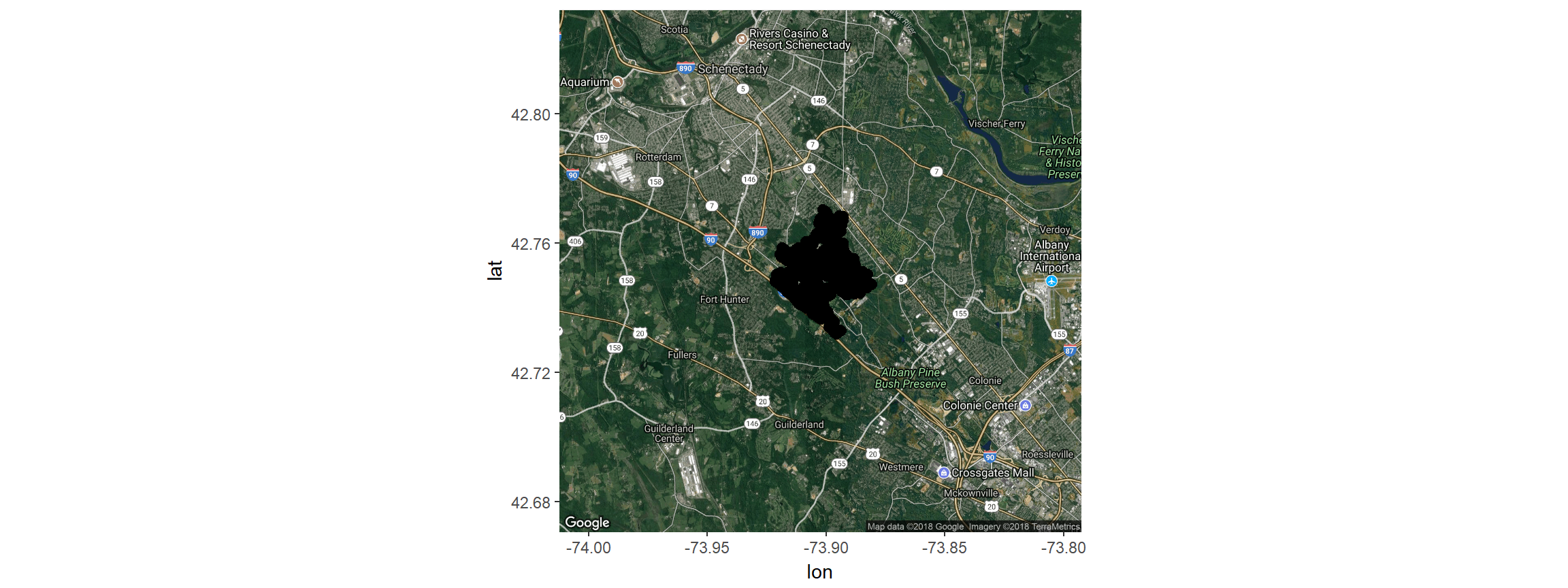

# plot the track on the map

Now, using leaflet

leaflet(fisherF2)%>%addTiles()%>%
  addCircles(fisherF2$location_long, fisherF2$location_lat)

Using ggplot without a background

Use separate axes for each individual (add scales=“free” to facet_wrap)

ggplot(fisher.dat, aes(x=location_long, y=location_lat))+geom_point()+
  facet_wrap(~local_identifier, scales="free")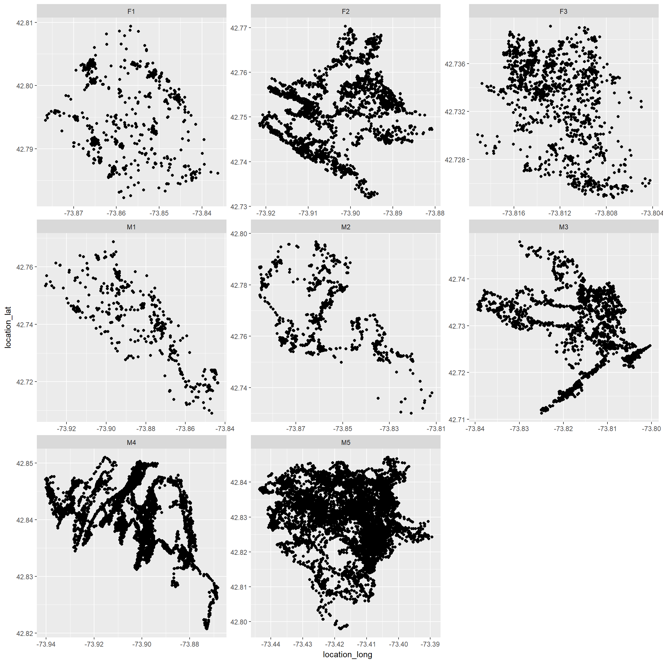

Now, all on 1 plot

ggplot(fisher.dat, aes(x=location_long, y=location_lat, color=as.factor(local_identifier)))+
  geom_point()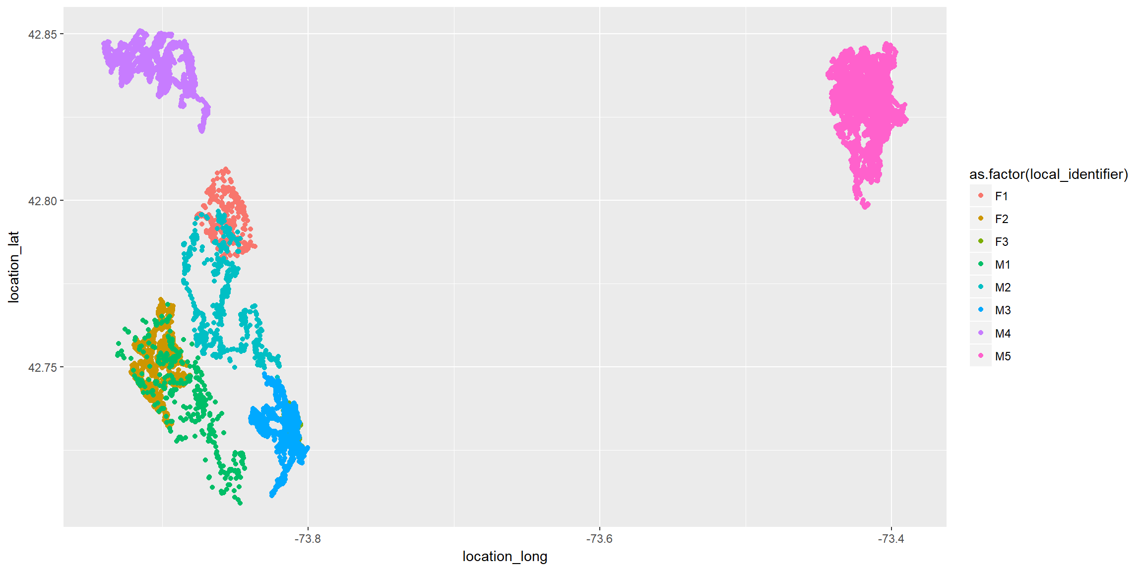

Creating a track in amt

Before we can use the amt package to calculate step lengths, turn angles, and bearings for fisher data, we need to add a class (track) to the data. Then, we can summarize the data by individual, month, etc. First, create a track using utms and the timestamp.

If we have a data set with locations in utms, we could use:

#trk.temp <- make_track(fisher.dat, .x=utm.easting, .y=utm.northing, .t=timestamp, id = individual_local.identifier)
#trk.temp

Note: we did not need to explicitly specify x, y and t (but probably good to do so). This would also have worked trk <- make_track(fisher.dat, utm.easting, utm.northing, timestamp, id = local_identifier) We can also use lat, long, which will allow us to determine time of day

trk <- mk_track(fisher.dat, .x=location_long, .y=location_lat, .t=timestamp, id = local_identifier, 
                crs = CRS("+init=epsg:4326"))

## .t found, creating `track_xyt`.

# Now it is easy to calculate day/night with either movement track
trk <- trk %>% time_of_day()

Now, we can transform back to geographic coordinates

trk <- transform_coords(trk, CRS("+init=epsg:32618"))

If we create trk.temp as above, we can make sure that we got back the same coordinates by comparing to the original track

#mean(trk$x_ - trk.temp$x_) # look good, there is virtually no difference
#mean(trk$y_ - trk.temp$y_) # same for y

Save the class here (and apply it later after adding columns to the object)

trk.class<-class(trk)

Movement Characteristics

dir_abs will calculate absolute angles for steps
dir_rel will calculate turning angles (relative angles)
step_lengths will calculate distances between points
nsd = Net Squared Displacement (distance from first point)

Arguments direction_abs:

full_circle will calculate between 0 and 360 (rather than -180 and 180)
zero gives the direction = 0 for absolute angle

Note: we have to calculate these characteristics separately for each individual (to avoid calculating a distance between say the last observation of the first individual and the first observation of the second individual).

To do this, we could loop through individuals, calculate these characteristics for each individual, then rbind the data back together. Or, use nested data frames and the map function in the purrr library to do this with very little code.

To see how nesting works, we can create a nested object by individual

nesttrk<-trk%>%nest(-id)
nesttrk

## # A tibble: 8 x 2
##   id    data                 
##   <fct> <list>               
## 1 M1    <tibble [919 x 4]>   
## 2 M4    <tibble [8,958 x 4]> 
## 3 F2    <tibble [3,004 x 4]> 
## 4 M3    <tibble [2,436 x 4]> 
## 5 F3    <tibble [1,501 x 4]> 
## 6 M2    <tibble [1,638 x 4]> 
## 7 F1    <tibble [1,349 x 4]> 
## 8 M5    <tibble [13,099 x 4]>

Each row contains data from an individual. For example, we can access data from the first individual using:

nesttrk$data[[1]]

## # A tibble: 919 x 4
##         x_       y_ t_                      tod_ 
##  *   <dbl>    <dbl> <dttm>                  <chr>
##  1 590130. 4732942. 2009-02-11 12:16:45.000 day  
##  2 590136. 4732940. 2009-02-11 12:31:38.000 day  
##  3 590138. 4732935. 2009-02-11 12:45:48.997 day  
##  4 590144. 4732947. 2009-02-11 13:00:16.002 day  
##  5 590137. 4732940. 2009-02-11 13:15:19.000 day  
##  6 590126. 4732936. 2009-02-11 13:30:13.000 day  
##  7 590139. 4732941. 2009-02-11 13:45:37.000 day  
##  8 590139. 4732923. 2009-02-11 14:00:35.000 day  
##  9 590137. 4732934. 2009-02-11 14:15:49.000 day  
## 10 590136. 4732935. 2009-02-11 14:30:49.000 day  
## # ... with 909 more rows

We could calculate movement characteristics by individual using:

temp<-direction_rel(nesttrk$data[[1]])
head(temp)

## [1]        NA -55.96892 130.93489 159.69985 -24.84488 179.16947

or:

temp<-trk %>% filter(id=="M1") %>% direction_rel
head(temp)

## [1]        NA -55.96892 130.93489 159.69985 -24.84488 179.16947

Or, we can add a columns to each nested column of data using purrr::map

trk<-trk %>% nest(-id) %>% 
  mutate(dir_abs = map(data, direction_abs,full_circle=TRUE, zero="N"), 
         dir_rel = map(data, direction_rel), 
         sl = map(data, step_lengths),
         nsd_=map(data, nsd))%>%unnest()

Now, calculate month, year, hour, week of each observation and append these to the dataset Unlike the movement charactersitics, these calculations can be done all at once, since they do not utilize successive observations (like step lengths and turn angles do).

trk<-trk%>% 
  mutate(
    week=week(t_),
    month = month(t_, label=TRUE), 
    year=year(t_),
    hour = hour(t_)
  )

Now, we need to again tell R that this is a track (rather than just a data frame)

class(trk)

## [1] "tbl_df"     "tbl"        "data.frame"

class(trk)<-trk.class

Lets take a look at what we created

trk

## # A tibble: 32,904 x 13
##    id    dir_abs dir_rel    sl  nsd_      x_       y_ t_                      tod_   week month  year  hour
##    <fct>   <dbl>   <dbl> <dbl> <dbl>   <dbl>    <dbl> <dttm>                  <chr> <dbl> <ord> <dbl> <int>
##  1 M1      259.     NA    6.38   0   590130. 4732942. 2009-02-11 12:16:45.000 day       6 Feb    2009    12
##  2 M1      203.    -56.0  5.61  40.7 590136. 4732940. 2009-02-11 12:31:38.000 day       6 Feb    2009    12
##  3 M1      334.    131.  12.7  112.  590138. 4732935. 2009-02-11 12:45:48.997 day       6 Feb    2009    12
##  4 M1      134.    160.   9.65 222.  590144. 4732947. 2009-02-11 13:00:16.002 day       6 Feb    2009    13
##  5 M1      109.    -24.8 11.7   52.2 590137. 4732940. 2009-02-11 13:15:19.000 day       6 Feb    2009    13
##  6 M1      288.    179.  13.9   46.1 590126. 4732936. 2009-02-11 13:30:13.000 day       6 Feb    2009    13
##  7 M1      180.   -109.  17.3   85.5 590139. 4732941. 2009-02-11 13:45:37.000 day       6 Feb    2009    13
##  8 M1       13.0  -167.  10.5  419.  590139. 4732923. 2009-02-11 14:00:35.000 day       6 Feb    2009    14
##  9 M1       34.7    21.7  1.57 111.  590137. 4732934. 2009-02-11 14:15:49.000 day       6 Feb    2009    14
## 10 M1      317.    -77.8  7.51  80.7 590136. 4732935. 2009-02-11 14:30:49.000 day       6 Feb    2009    14
## # ... with 32,894 more rows

Some plots of movement characteristics

Absolute angles (for each movement) relative to North

We could use a rose diagram (below) to depict the distribution of angles.

ggplot(trk, aes(x = dir_abs, y=..density..)) + geom_histogram(breaks = seq(0,360, by=20))+
  coord_polar(start = 0) + theme_minimal() + 
  scale_fill_brewer() + ylab("Density") + ggtitle("Angles Direct") + 
  scale_x_continuous("", limits = c(0, 360), breaks = seq(0, 360, by=20), 
                     labels = seq(0, 360, by=20))+
  facet_wrap(~id)

## Warning: Removed 8 rows containing non-finite values (stat_bin).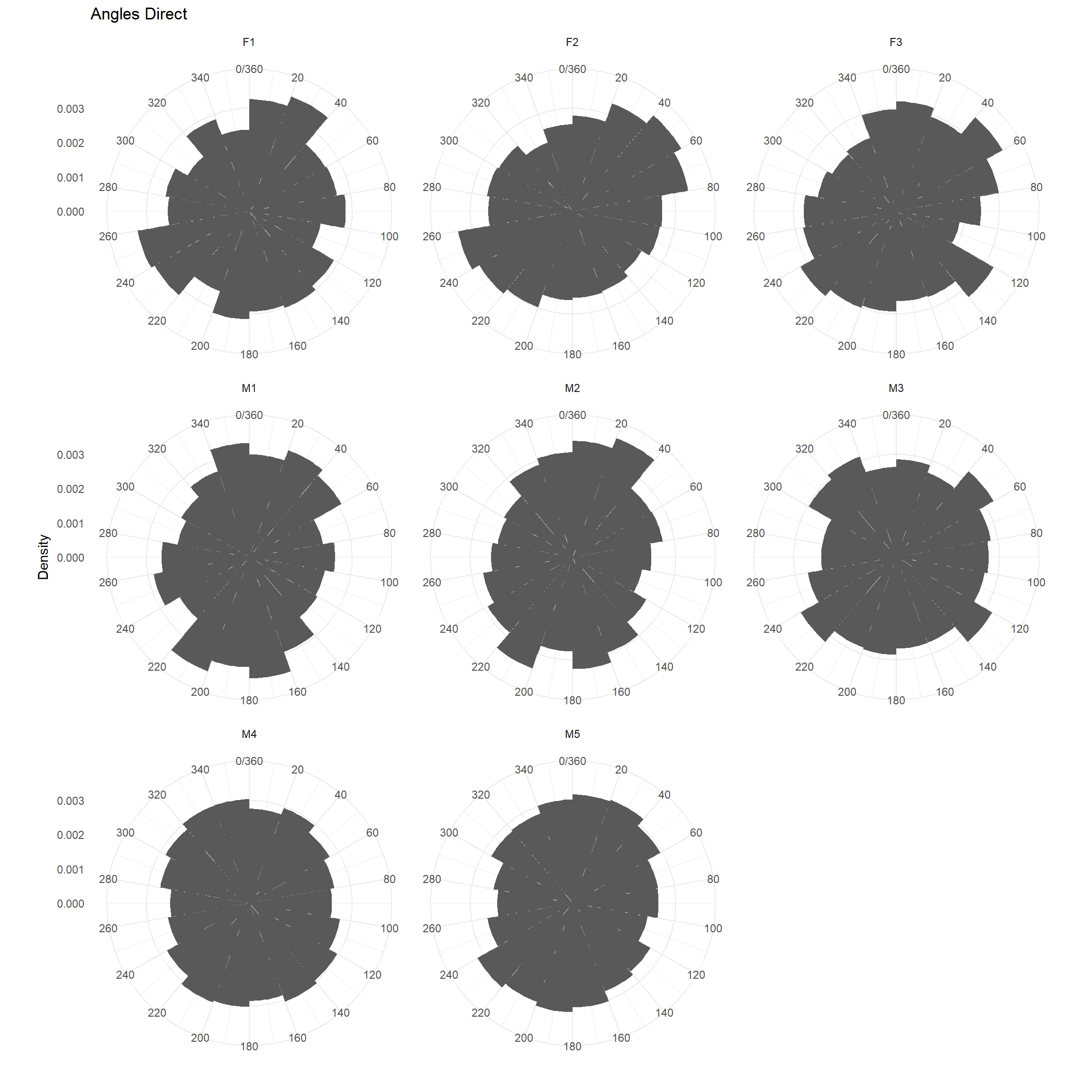

Turning angles

Note: a 0 indicates the animal continued to move in a straight line, a 180 indicates the animal turned around (but note, resting + measurement error often can make it look like the animal turned around).

ggplot(trk, aes(x = dir_rel, y=..density..)) + geom_histogram(breaks = seq(-180,180, by=20))+
  coord_polar(start = 0) + theme_minimal() + 
  scale_fill_brewer() + ylab("Density") + ggtitle("Angles Direct") + 
  scale_x_continuous("", limits = c(-180, 180), breaks = seq(-180, 180, by=20), 
                     labels = seq(-180, 180, by=20))+
  facet_wrap(~id)

## Warning: Removed 16 rows containing non-finite values (stat_bin).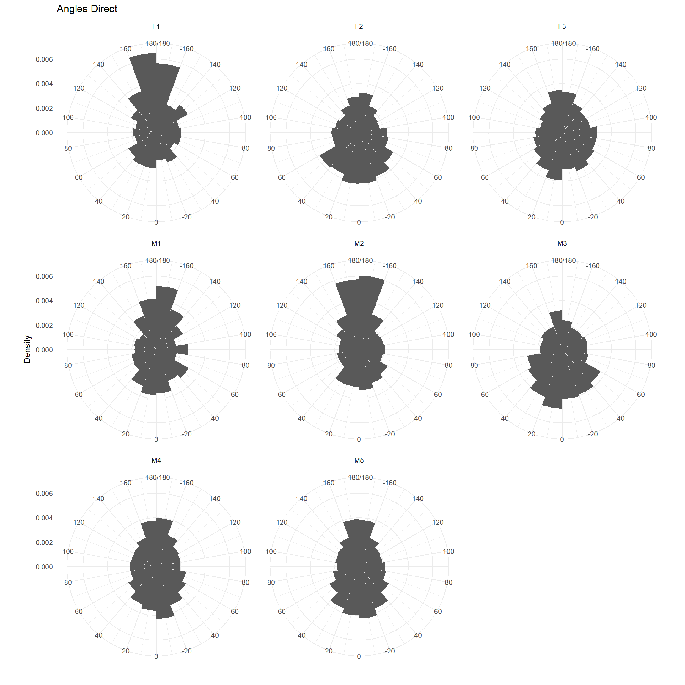

Turning angles as histograms

ggplot(trk, aes(x = dir_rel)) +  geom_histogram(breaks = seq(-180,180, by=20))+
  theme_minimal() + 
  scale_fill_brewer() + ylab("Count") + ggtitle("Angles Relative") + 
  scale_x_continuous("", limits = c(-180, 180), breaks = seq(-180, 180, by=20),
                     labels = seq(-180, 180, by=20))+facet_wrap(~id, scales="free")

## Warning: Removed 16 rows containing non-finite values (stat_bin).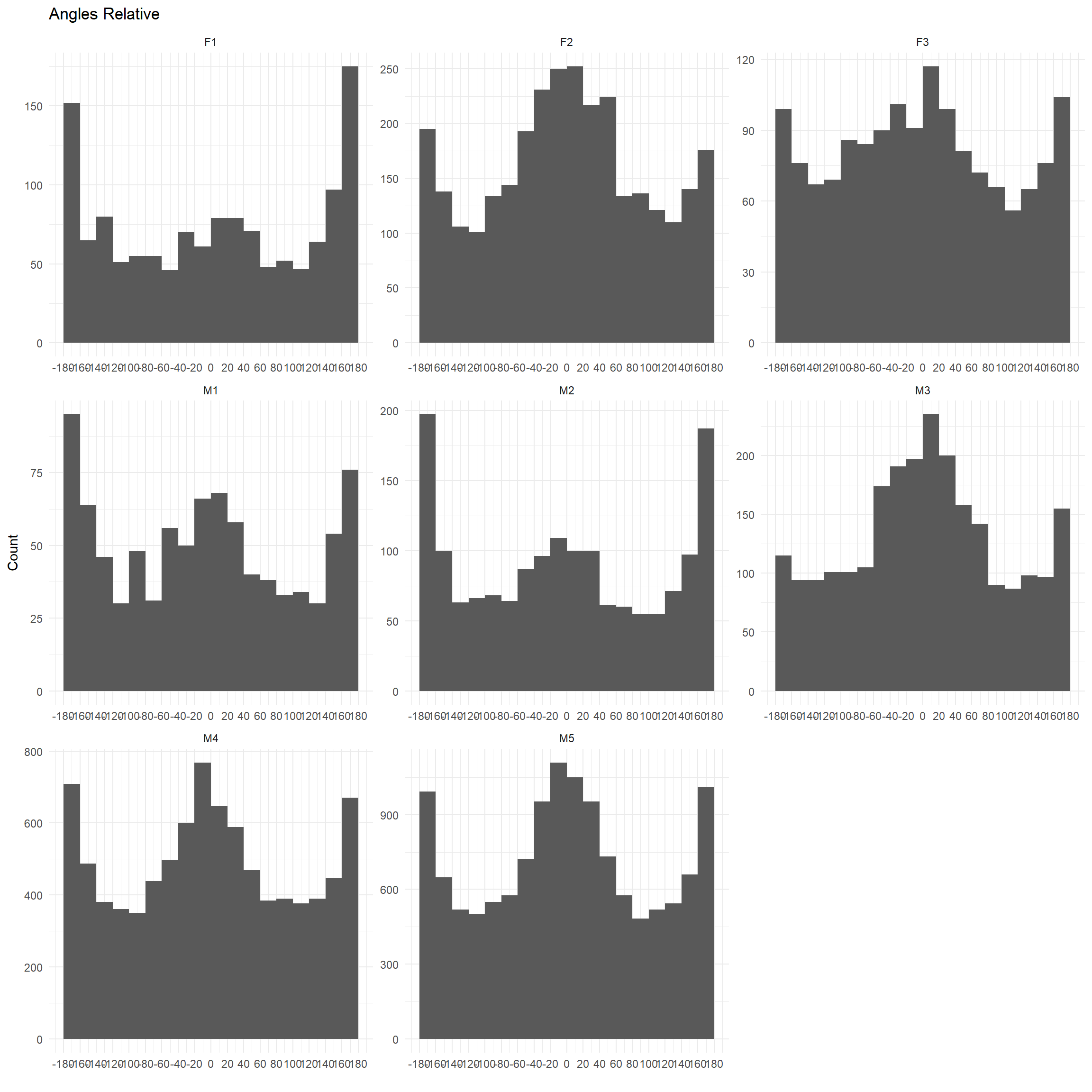

Net-squared displacement over time for each individual

ggplot(trk, aes(x = t_, y=nsd_)) + geom_point()+
  facet_wrap(~id, scales="free")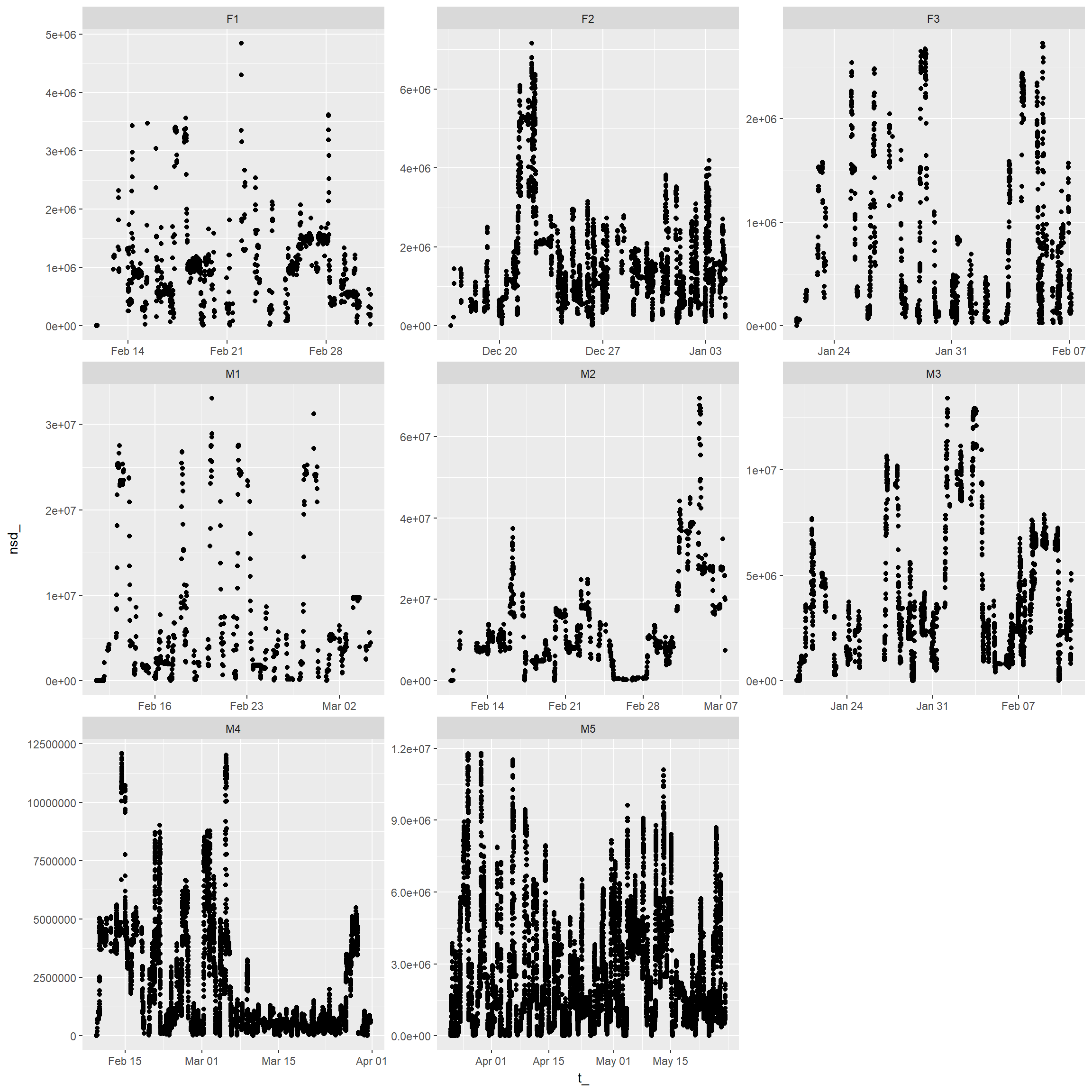

Explore movement characteristics by (day/night, hour, month)

step length distribution by day/night

ggplot(trk, aes(x = tod_, y = log(sl))) + 
  geom_boxplot()+geom_smooth()+facet_wrap(~id)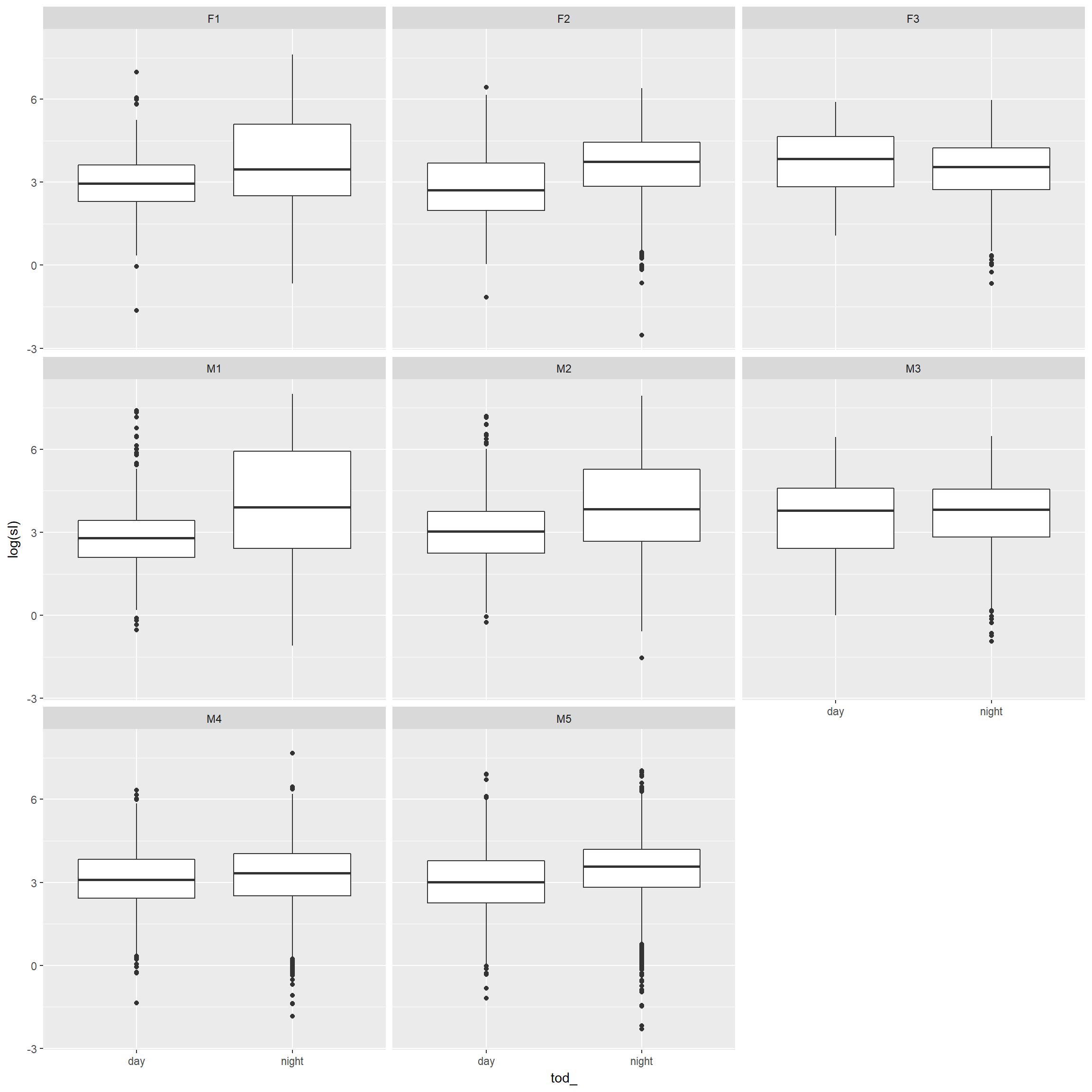

Space use (MCP or KDE) by week, month, and year

Note: this code will only work for your critters if you have multiple observations for each combination of (month, year). If you don’t have many observations, you could try: nest(-id, -year) and unnest(id,year)

mcps.week<-trk %>% nest(-id,-year,  -month, -week) %>%  
  mutate(mcparea = map(data, ~hr_mcp(., levels = c(0.95)) %>% hr_area)) %>% 
  select(id, year, month, week, mcparea) %>% unnest()

ggplot(mcps.week, aes(x = week, y = area, colour=as.factor(year))) + geom_point()+
  geom_smooth()+ facet_wrap(~id, scales="free")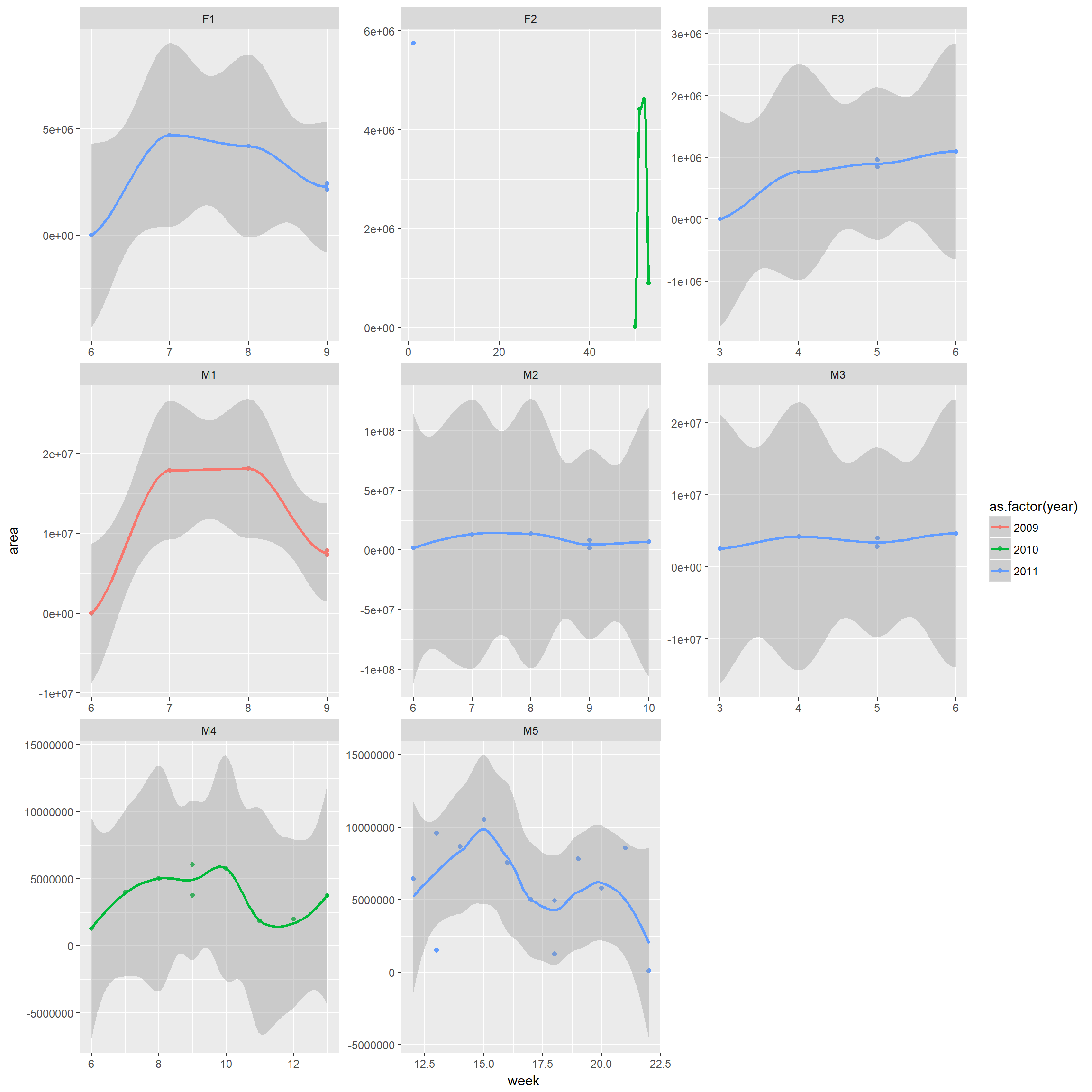

Same for KDE

kde.week<-trk %>% nest(-id,-year,  -month, -week) %>%  
  mutate(kdearea = map(data, ~hr_kde(., levels=c(0.95)) %>% hr_area)) %>%
  select(id, year, month, week,  kdearea) %>% unnest()

ggplot(kde.week, aes(x = week, y = kdearea, colour=as.factor(year))) + geom_point()+
  geom_smooth()+ facet_wrap(~id, scales="free")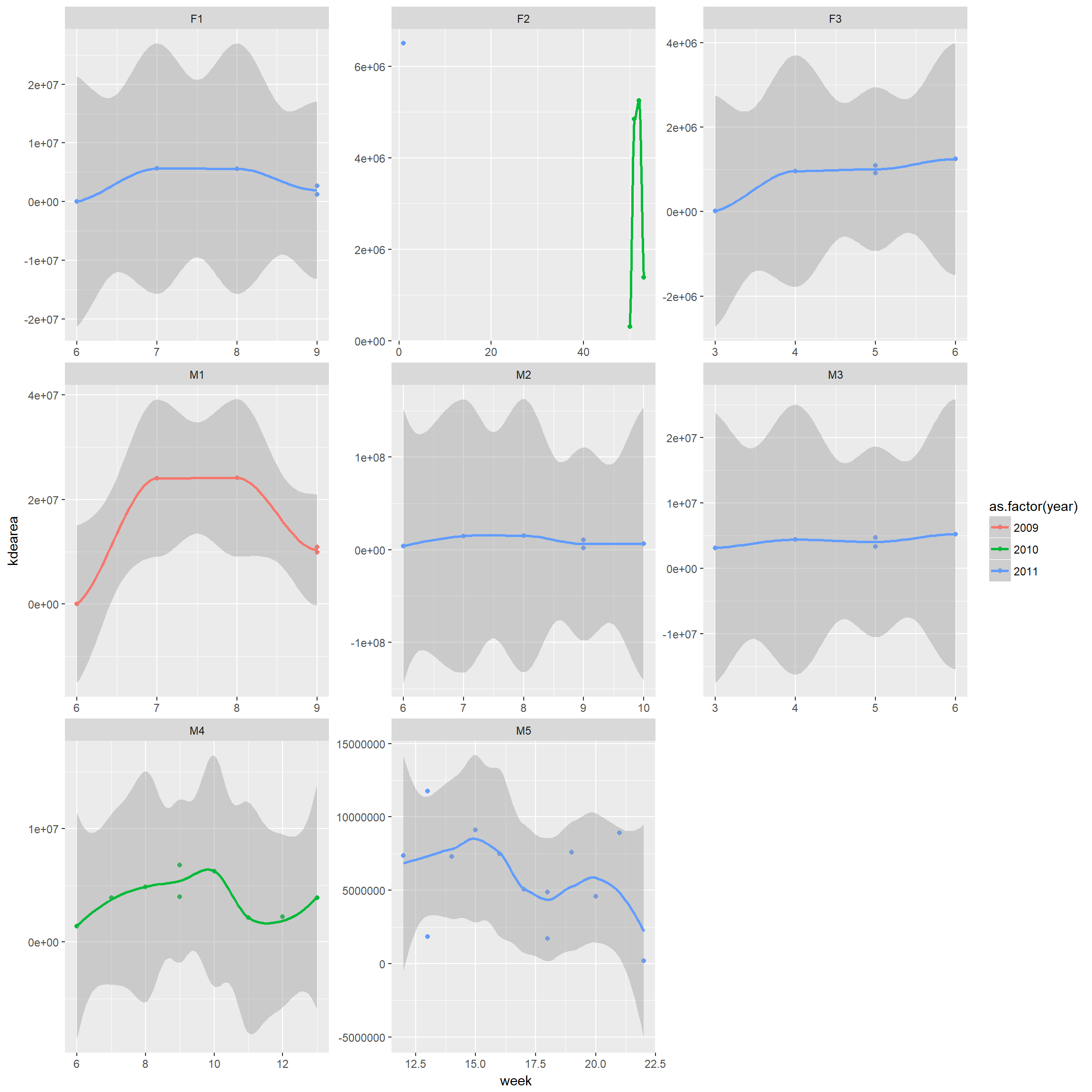

RSF prep

Generate random points within MCPs for a single individual using amt functions. Notes:

It is common to generate points randomly, but other options are possible.
In particular, it can beneficial to generate a systematically placed sample
Samples can also be generated using the spsample function in the sp library or using a GIS (note: amt uses the spsample function within its function random_points)
Other home range polygons could be used (e.g., kernel density, local convex hull etc.)

Random points: illustrate for 1 individual

trk %>% filter(id=="F1") %>%
  random_points(.,factor = 20) %>% plot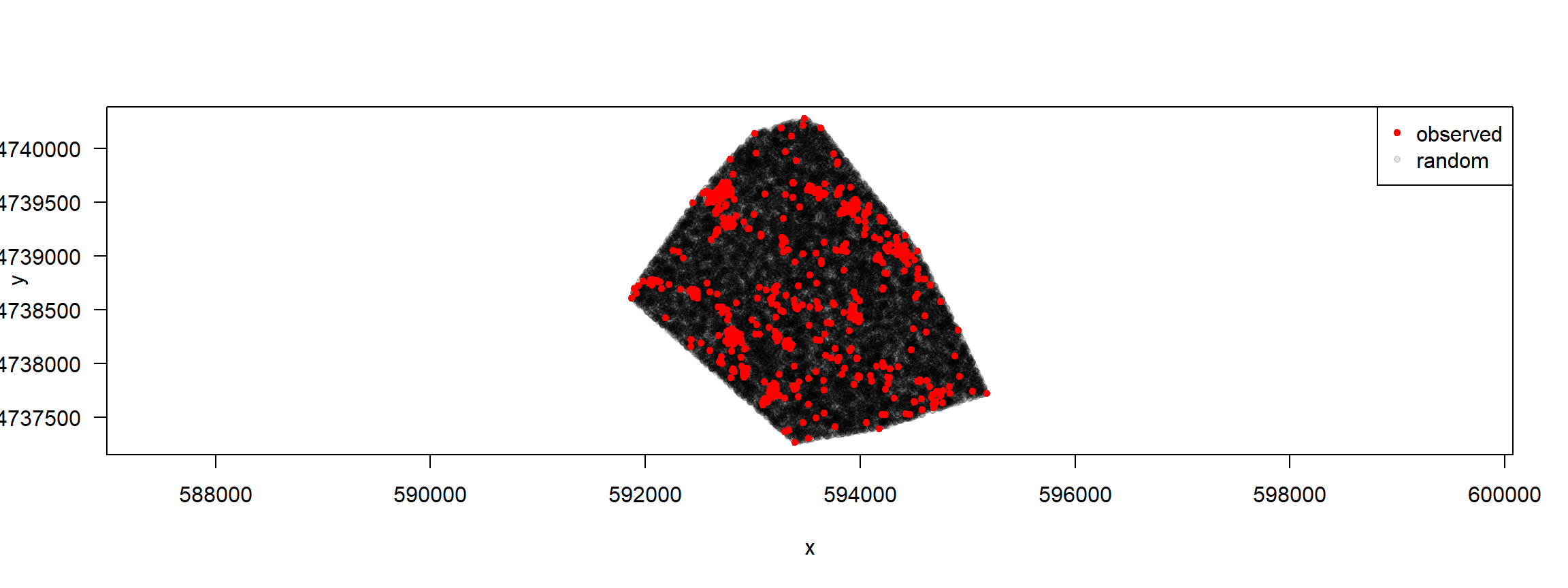

Illustrate systematic points (to do this, we need to create the mcp first)

trk%>%filter(id=="F1") %>% 
  random_points(., factor = 20, type="regular") %>% 
  plot()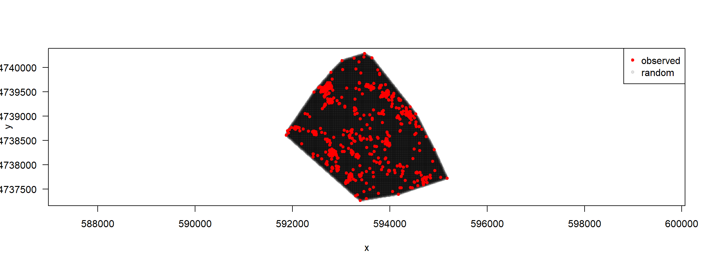

Now, lets generate points for all individuals. We can do this efficiently by making use of pipes (%>%),nested data frames, and then by adding a new column – a list-column – to trks

avail.pts <- trk %>% nest(-id) %>% 
  mutate(rnd_pts = map(data, ~ random_points(., factor = 20, type="regular"))) %>% 
  select(id, rnd_pts) %>%  # you dont want to have the original point twice, hence drop data
  unnest()

Or, we could do this using a loop (commented out, below)

#avail.pts<-NULL
#uid<-unique(trk$id) # individual identifiers
#luid<-length(uid) # number of unique individuals
#for(i in 1:luid){
# random_points will generate random points within mcp
# Add on the individual id and combine all data
#  temp<-cbind(id=uid[i],trk%>%filter(id==uid[i])%>%random_points)
#  avail.pts<-rbind(avail.pts, temp)
#}
#avail.pts<-as_tibble(avail.pts)
#avail.pts

Write out data for further annotating

Need to rename variables so everything is in the format Movebank requires for annotation of generic time-location records (see https://www.movebank.org/node/6608#envdata_generic_request). This means, we need the following variables:

location-lat (perhaps with addition of Easting/Northing in UTMs)
location-long (perhaps with addition of Easting/Northing in UTMs)
timestamp (in Movebank format)

Need to project to lat/long, while also keeping lat/long. Then rename variables and write out the data sets.

avail <- SpatialPointsDataFrame(avail.pts[,c("x_","y_")], avail.pts, 
                                proj4string=CRS("+proj=utm +zone=18N +datum=WGS84"))  
avail.df <- data.frame(spTransform(avail, CRS("+proj=longlat +datum=WGS84")))[,1:6]
names(avail.df)<-c("idr", "case_", "utm.easting", "utm.northing", "location-long", "location-lat")

Check to make sure everything looks right

test<-subset(avail.df, case_==TRUE)
test %>% select('location-lat', 'location-long', utm.easting, utm.northing) %>% 
  summarise_all(mean)

##   location-lat location-long utm.easting utm.northing
## 1     42.80687     -73.69359    606812.2      4740221

fisher.dat %>% summarize(meanloc.lat=mean(location_lat), 
                         meanloc.long=mean(location_long))

##   meanloc.lat meanloc.long
## 1    42.80687    -73.69359

Add a timestamp to annotate these data with environmental covariates in Movebank using Env-DATA (https://www.movebank.org/node/6607). Here we just use the first timestamp, however meaningful timestamps are needed if annotating variables that vary in time.

avail.df$timestamp<-fisher.dat$timestamp[1]

These points then need to be annotated prior to fitting rsfs. Let’s write out 2 files:

FisherRSF2018.csv will contain all points and identifying information.
FisherRSFannotate.csv will contain only the columns used to create the annotation.

The latter file will take up less space, making it easier to annotate (and also possible to upload to github)

write.csv(avail.df, file="data/FisherRSF2018.csv", row.names = FALSE)

avail.df<-avail.df %>% select("timestamp", "location-long", "location-lat")
write.csv(avail.df, file="data/FisherRSFannotate.csv", row.names = FALSE)

SSF prep

SSFs assume that data have been collected at regular time intervals. We can use the track_resample function to regularize the trajectory so that all points are located within some tolerence of each other in time. To figure out a meaningful tolerance range, we should calculate time differences between locations & look at as a function of individual.

(timestats<-trk %>% nest(-id) %>% mutate(sr = map(data, summarize_sampling_rate)) %>%
    select(id, sr) %>% unnest)

## # A tibble: 8 x 10
##   id        min    q1 median  mean    q3   max    sd     n unit 
##   <fct>   <dbl> <dbl>  <dbl> <dbl> <dbl> <dbl> <dbl> <int> <chr>
## 1 M1    13.3    14.7   15.0  32.7  15.5   977. 104.    918 min  
## 2 M4     0.1000  1.93   2.03  8.04  2.57 1209.  44.0  8957 min  
## 3 F2     0.400   1.97   2.03  8.93  3.98 1080.  48.1  3003 min  
## 4 M3     0.417   1.97   2.17 13.3   5.42 2889.  90.2  2435 min  
## 5 F3     0.417   1.97   2.07 15.7   4.08 2167. 104.   1500 min  
## 6 M2     1.35    9.78  10.0  21.7  10.3  2111.  87.2  1637 min  
## 7 F1     3.92    9.80  10.0  20.7  10.3  1650.  95.2  1348 min  
## 8 M5     0.250   1.93   2.02  7.41  2.37  976.  25.0 13098 min

Time intervals range from every 2 to 15 minutes on average, depending on the individual. Lets add on the time difference to each obs.

trk<-trk %>% group_by(id) %>% mutate(dt_ = t_ - lag(t_, default = NA))

Let’s illustrate track regularization with ID = F2. Let’s go from every 2 minutes to every 10.

tempF2<-trk %>% filter(id=="F2") %>% track_resample(rate=minutes(10), tolerance=minutes(2))
tempF2 %>% select(id, x_, y_, t_, burst_)

## # A tibble: 1,010 x 5
## # Groups:   id [1]
##    id         x_       y_ t_                      burst_
##  * <fct>   <dbl>    <dbl> <dttm>                   <dbl>
##  1 F2    590028. 4733219. 2010-12-16 16:45:30.999      1
##  2 F2    590486. 4733344. 2010-12-16 21:21:13.999      2
##  3 F2    591220. 4733065. 2010-12-16 21:32:34.000      2
##  4 F2    591215. 4733037. 2010-12-17 08:57:00.999      3
##  5 F2    591172. 4733057. 2010-12-17 09:05:14.000      3
##  6 F2    591075. 4733081. 2010-12-17 09:16:29.000      3
##  7 F2    591024. 4733025. 2010-12-17 09:24:53.000      3
##  8 F2    590793. 4732994. 2010-12-17 09:37:24.000      4
##  9 F2    590838. 4733077. 2010-12-18 01:08:42.997      5
## 10 F2    590658. 4733176. 2010-12-18 01:24:34.000      6
## # ... with 1,000 more rows

Now loop over individuals and do the following:

Regularize trajectories using an appropriate time window (see e.g., below)
calculate new dt values
Create bursts using individual-specific time intervals
Generate random steps within each burst

The random steps are generated using the following approach:

Fit a gamma distribution to step lenghts
Fit a von mises distribution to turn angles
Use these distribution to draw new turns and step lengths, form new simulated steps and generate random x,y values.

ssfdat<-NULL
temptrk<-with(trk, track(x=x_, y=y_, t=t_, id=id))
uid<-unique(trk$id) # individual identifiers
luid<-length(uid) # number of unique individuals
for(i in 1:luid){
  # Subset individuals & regularize track
  temp<-temptrk%>% filter(id==uid[i]) %>% 
    track_resample(rate=minutes(round(timestats$median[i])), 
                   tolerance=minutes(max(10,round(timestats$median[i]/5))))
  
  # Get rid of any bursts without at least 2 points
  temp<-filter_min_n_burst(temp, 2)
  
  # burst steps
  stepstemp<-steps_by_burst(temp)
  
  # create random steps using fitted gamma and von mises distributions and append
  rnd_stps <- stepstemp %>%  random_steps(n = 15)
  
  # append id
  rnd_stps<-rnd_stps%>%mutate(id=uid[i])
  
  # append new data to data from other individuals
  ssfdat<-rbind(rnd_stps, ssfdat)
}
ssfdat<-as_tibble(ssfdat)
ssfdat

## # A tibble: 470,000 x 13
##    burst_ step_id_ case_     x1_      y1_     x2_      y2_ t1_                     t2_                     dt_       sl_    ta_ id   
##     <dbl>    <int> <lgl>   <dbl>    <dbl>   <dbl>    <dbl> <dttm>                  <dttm>                  <time>  <dbl>  <dbl> <fct>
##  1      1        1 TRUE  630498. 4742879. 630569. 4742823. 2011-03-22 00:02:12.997 2011-03-22 00:04:10.997 118     90.4   -62.6 M5   
##  2      1        1 FALSE 630498. 4742879. 630531. 4742824. 2011-03-22 00:02:12.997 2011-03-22 00:04:10.997 118     33.3  -113.  M5   
##  3      1        1 FALSE 630498. 4742879. 630509. 4742929. 2011-03-22 00:02:12.997 2011-03-22 00:04:10.997 118    107.   -130.  M5   
##  4      1        1 FALSE 630498. 4742879. 630500. 4742826. 2011-03-22 00:02:12.997 2011-03-22 00:04:10.997 118      3.90 -125.  M5   
##  5      1        1 FALSE 630498. 4742879. 630506. 4742823. 2011-03-22 00:02:12.997 2011-03-22 00:04:10.997 118      7.73   50.2 M5   
##  6      1        1 FALSE 630498. 4742879. 630473. 4742855. 2011-03-22 00:02:12.997 2011-03-22 00:04:10.997 118     40.4    77.6 M5   
##  7      1        1 FALSE 630498. 4742879. 630526. 4742862. 2011-03-22 00:02:12.997 2011-03-22 00:04:10.997 118     48.2  -150.  M5   
##  8      1        1 FALSE 630498. 4742879. 630574. 4742643. 2011-03-22 00:02:12.997 2011-03-22 00:04:10.997 118    195.    143.  M5   
##  9      1        1 FALSE 630498. 4742879. 630534. 4742723. 2011-03-22 00:02:12.997 2011-03-22 00:04:10.997 118    107.     80.5 M5   
## 10      1        1 FALSE 630498. 4742879. 630495. 4742822. 2011-03-22 00:02:12.997 2011-03-22 00:04:10.997 118      3.41   28.8 M5   
## # ... with 469,990 more rows

Now, lets plot the data for random and matched points

ggplot(ssfdat, aes(x2_, y2_, color=case_))+geom_point()+facet_wrap(~id, scales="free")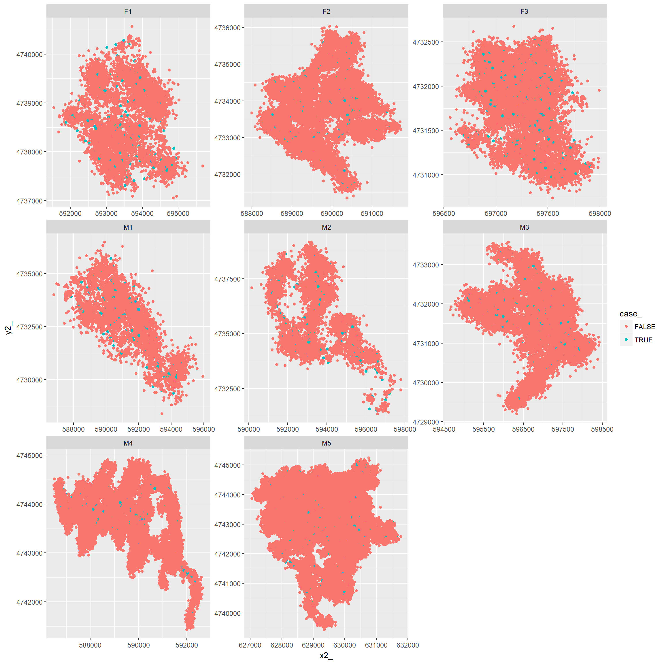

Relabel as utms

ssfdat$utm.easting<-ssfdat$x2_
ssfdat$utm.northing<-ssfdat$y2_

Write out data for further annotating

location-lat (perhaps with addition of Easting/Northing in UTMs)
location-long (perhaps with addition of Easting/Northing in UTMs)
timestamp (in Movebank format)

Need to project to lat/long, while also keeping lat/long. Then rename variables and write out the data sets. With the SSFs, we have the extra complication of having a time and location at both the start and end of the step.

For the time being, we will assume we want to annotate variables at the end of the step but use the starting point of the step as the timestamp.

You could also calculate the midpoint of the timestep like this: data$timestamp.midpoint <- begintime + (endtime-begintime)/2

ssfdat2 <- SpatialPointsDataFrame(ssfdat[,c("x2_","y2_")], ssfdat, 
                                  proj4string=CRS("+proj=utm +zone=18N +datum=WGS84"))  
ssf.df <- data.frame(spTransform(ssfdat2, CRS("+proj=longlat +datum=WGS84"))) 
names(ssf.df)[c(13,16,17)] <-c("individual.local.identifier", "location-long", "location-lat")
ssf.df$timestamp<-ssf.df$t1_
ssf.df %>% select('location-lat', utm.easting, x1_, x2_, y1_, y2_, 'location-long', utm.northing) %>% head

##   location-lat utm.easting      x1_      x2_     y1_     y2_ location-long utm.northing
## 1     42.82684    630568.9 630497.9 630568.9 4742879 4742823     -73.40259      4742823
## 2     42.82685    630531.2 630497.9 630531.2 4742879 4742824     -73.40305      4742824
## 3     42.82780    630509.4 630497.9 630509.4 4742879 4742929     -73.40329      4742929
## 4     42.82688    630500.4 630497.9 630500.4 4742879 4742826     -73.40342      4742826
## 5     42.82685    630505.6 630497.9 630505.6 4742879 4742823     -73.40336      4742823
## 6     42.82714    630472.7 630497.9 630472.7 4742879 4742855     -73.40375      4742855

These points then need to be annotated prior to fitting ssfs. Let’s write out 2 files:

FisherSSF2018.csv will contain all points and identifying information.
FisherSSFannotate.csv will contain only the columns used to create the annotation.

The latter file will take up less space, making it easier to annotate (and also possible to upload to github)

write.csv(ssf.df, file="data/AllStepsFisher2018.csv", row.names=FALSE)
ssf.df<-ssf.df %>% select("timestamp", "location-long", "location-lat")
write.csv(ssf.df, file="data/FisherSSFannotate.csv", row.names = FALSE)

Using nested data frames

This works if all animals are sampled at a constant sampling rate. Again, you need to create a new column (using mutate) where you save the random steps to Not all animals have a 15 min sampling rate, so we might drop the first animal that has a 15 minute sampling rate.

#trk %>% nest(-id) %>% mutate(sr = map(.$data, summarize_sampling_rate)) %>% 
#  select(id, sr) %>% unnest()

# Then, we could avoid a loop with:
#ssfdat <- trk %>% filter(id != "M1") %>% nest(-id) %>% 
#  mutate(ssf = map(data, function(d) {
#    d %>%
#      track_resample(rate = minutes(10), tolerance = minutes(2)) %>% 
#      filter_min_n_burst(min_n = 3) %>% 
#      steps_by_burst() %>% random_steps()
#  })) %>% select(id, ssf) %>% unnest()

Document Footer

Session Information:

sessionInfo()

## R version 3.5.0 (2018-04-23)
## Platform: x86_64-w64-mingw32/x64 (64-bit)
## Running under: Windows >= 8 x64 (build 9200)
## 
## Matrix products: default
## 
## locale:
## [1] LC_COLLATE=English_United States.1252  LC_CTYPE=English_United States.1252    LC_MONETARY=English_United States.1252 LC_NUMERIC=C                          
## [5] LC_TIME=English_United States.1252    
## 
## attached base packages:
## [1] stats     graphics  grDevices utils     datasets  methods   base     
## 
## other attached packages:
##  [1] bindrcpp_0.2.2  dplyr_0.7.4     leaflet_2.0.0   tibble_1.4.2    ggmap_2.6.1     ggplot2_2.2.1   amt_0.0.4.0     move_3.0.2      rgdal_1.2-18    geosphere_1.5-7
## [11] raster_2.6-7    maptools_0.9-2  sp_1.2-7        lubridate_1.7.4 knitr_1.20     
## 
## loaded via a namespace (and not attached):
##  [1] httr_1.3.1         maps_3.3.0         tidyr_0.8.0        jsonlite_1.5       splines_3.5.0      shiny_1.0.5        assertthat_0.2.0   yaml_2.1.19       
##  [9] pillar_1.2.2       backports_1.1.2    lattice_0.20-35    glue_1.2.0         digest_0.6.15      promises_1.0.1     colorspace_1.3-2   htmltools_0.3.6   
## [17] httpuv_1.4.1       Matrix_1.2-14      plyr_1.8.4         pkgconfig_2.0.1    mvtnorm_1.0-7      purrr_0.2.4        xtable_1.8-2       scales_0.5.0      
## [25] jpeg_0.1-8         later_0.7.2        mgcv_1.8-23        lazyeval_0.2.1     cli_1.0.0          proto_1.0.0        survival_2.41-3    magrittr_1.5      
## [33] crayon_1.3.4       mime_0.5           evaluate_0.10.1    MASS_7.3-49        nlme_3.1-137       xml2_1.2.0         foreign_0.8-70     fitdistrplus_1.0-9
## [41] rsconnect_0.8.8    tools_3.5.0        RgoogleMaps_1.4.1  stringr_1.3.0      munsell_0.4.3      compiler_3.5.0     rlang_0.2.0        grid_3.5.0        
## [49] rjson_0.2.18       htmlwidgets_1.2    circular_0.4-93    crosstalk_1.0.0    labeling_0.3       rmarkdown_1.9      boot_1.3-20        gtable_0.2.0      
## [57] curl_3.2           reshape2_1.4.3     R6_2.2.2           rgeos_0.3-26       utf8_1.1.3         bindr_0.1.1        rprojroot_1.3-2    KernSmooth_2.23-15
## [65] stringi_1.1.7      parallel_3.5.0     Rcpp_0.12.16       mapproj_1.2.6      png_0.1-7          tidyselect_0.2.4

proc.time()-ptm

##    user  system elapsed 
##  109.92   58.38  186.76

TestVignette

John Fieberg

Purpose

Preamble

Data cleaning

Plots of the data

Using ggplot without a background

Creating a track in amt

Movement Characteristics

Some plots of movement characteristics

Absolute angles (for each movement) relative to North

Turning angles

Turning angles as histograms

Net-squared displacement over time for each individual

Explore movement characteristics by (day/night, hour, month)

step length distribution by day/night

Space use (MCP or KDE) by week, month, and year

RSF prep

Random points: illustrate for 1 individual

Write out data for further annotating

SSF prep

Write out data for further annotating

Using nested data frames

Document Footer